Source: Lucas Vieira (LucasVB), Wikimedia Commons

Mathematics

ABOUT: This is where I will post math projects, current interests/studies, and other cool finds I come across in the world of mathematics.

RELATED: Mathematics Book List

Table of Contents

• Rational Numbers Blog Post, 11/20/24
• Solving Kepler's Equation Numerically, 11/08/24
• Self-Teaching Differential Geometry, 08/19/24
• Venn Diagram of Mathematical Spaces, undated
• Calculus of Variations Analysis Seminar Presentation, undated
• Calculus of Variations Project, undated, incomplete

--- Rational Numbers Blog Post ---

11/20/2024

Over on my blog page I've written a sort of discussion about the limits of our physical knowledge of numbers titled "Rational Numbers Are All We Will Ever Know." I am not very good with titles, that is always the last thing I do. The premise is that we cannot measure things to arbitrary precision, and ultimately we can only ever describe the world using rational numbers. In fact, the larger portion of the reals, the irrationals, will never truly be a part of the real world. This likely mirrors a lot of other discussions of the question "are numbers real?" with the eventual answer of "no, but they give us a means to describe the world," much like with words. Words may not be real, only mental constructs, but the things they represent and convey certainly are real. Having said that, I do not make any claim that my conclusion is unique or original, but this is just my perspective on the specific case of whether or not real numbers are "real." I also use this as an opportunity to introduce the idea of the density of the rationals in the reals. I figured while I was on the topic of math I may as well sprinkle in something from set theory/analysis.

--- Solving Kepler's Equation via Iterative Numerical Methods---

11/08/2024

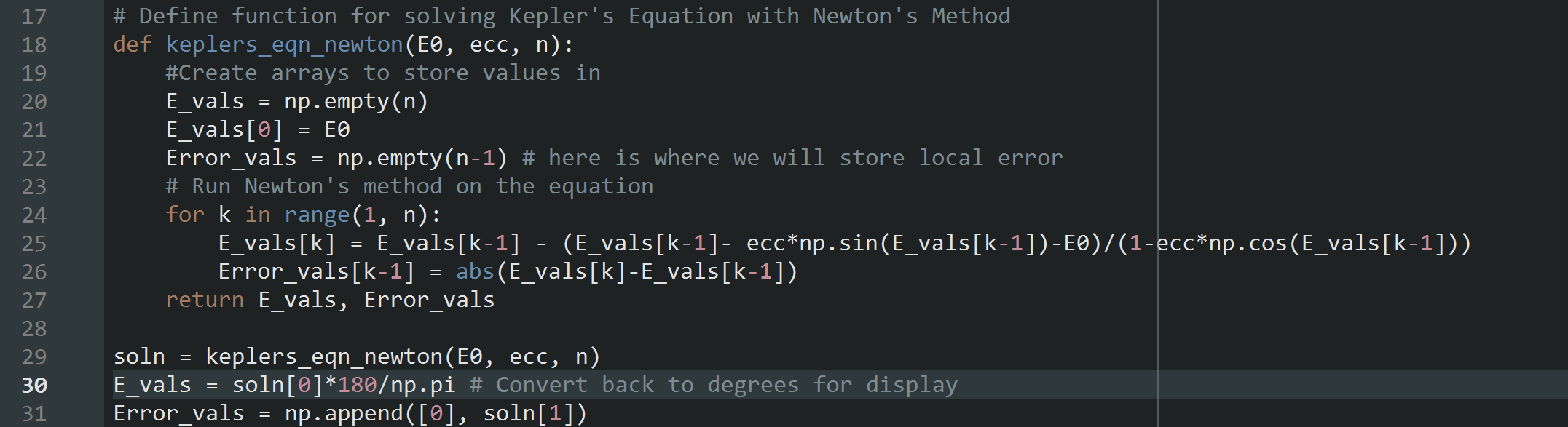
Awhile ago I was watching the video "Kepler's Impossible Equation" by Welch Labs on YouTube and before I got through it I wanted to try coding up the method described on my own. I have previous experience with numerical analysis in Python and Matlab, so I thought it could make for a fun project, but it turned out to be a good refresher in Python syntax too!

Kepler's equation is usually given as $M=E-e\sin (E)$. This allows us to find the position of a body in an elliptical orbit using just a couple parameters. I won't get into the weeds explaining the equation or the mechanics, but instead look at how to solve it numerically (there is actually no analytical solution to this seemingly simple equation!). If you are curious, the Wikipedia page does a wonderful job as one would expect. I chose to do this in Python since it is free and simple. You will need the Numpy and Pandas libraries too. The files I created are on my Github here.

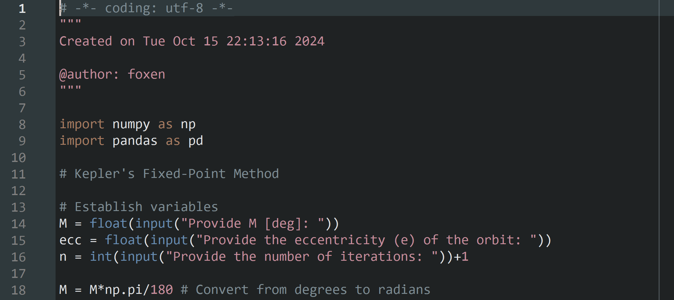
I created the code both in Spyder (a Python IDE for scientific computation) and using the notepad and the command line in Debian (more challenging but educational). Both work fine, but I will show it in Spyder here for clarity. Below is an image of the first steps in our code. We want to start the process by importing these two libraries into our code. We ask the user to input the parameters $M,e,$ and $n.$ These are the mean anomaly, orbital eccentricity, and number of iterations, respectively. I turned $M$ and $e$ (labeled "ecc" to avoid confusion with Euler's number) into float values since that solved error messsages and then kept $n$ as an integer (since it was trying to call it a string for some reason). It's important to specify for the user that $M$ has units of degrees since later we convert to radians (line 18).

From here we want to define a function that will run our fixed point iteration scheme. Before I discuss the code itself, I do want to look at fixed point iteration methods a bit. If you don't really care for the math, then skip to here.

Detour: Fixed Points and Iterative Methods

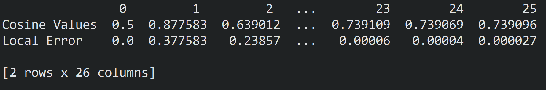
A fixed point of a function is a point where $f(x)=x.$ A prime example of this is the fixed point of cosine, called the Dottie number. This is the number where $\cos (x)=x$. You can find this yourself by repeatedly applying the cosine function to some given number. So for instance, let's take the number $0.5$ and plug it into cosine. We see $\cos (0.5)=0.877583\dots$ We take this number and plug it back into cosine as $\cos (0.877583)$ and get $0.639012\dots$ If you do this infinitely many times, the resulting values get infinitely close to the number $D=0.739085133\dots$ (Dottie's number). This behavior can be seen with just 25 iterations as shown below.

Many examples of fixed points exist and this behavior is critical to creating convergent numerical analysis schemes. There are also plenty of theorems that provide sufficient conditions for a fixed point to exist. One such theorem is the Banach Fixed Point Theorem. If you are familiar with analysis then there is a good chance you will have seen this before. If not, this is not necessary for the practical task of coding our solution and can be skipped if you'd like. First, it is important to define the term "contraction mapping." Given a metric space $(X,d)$, a function $T:X\to X$ is a contraction mapping if there exists a $k\in [0,1)$ such that $d(T(x),T(y))\le qd(x,y)$ for all $x,y\in X$. The theorem is as follows, from Wikipedia.

Banach Fixed Point Theorem

Let $(X,d)$ be a non-empty complete metric space and and $T:X\to X$ a contraction mapping. Then $T$ has a unique fixed point $x^{\ast }\in X$. The point $x^{\ast }$ can be found via the following method: choose an arbitrary $x_0\in X$ and define a sequence $(x_n{)}_{n\in \mathbb{N}}$ by $x_n=T(x_{n-1})$ for $n\ge 1.$ Then, $\underset{n\to \mathrm{\infty }}{lim}(x_n)=x^{\ast }.$

Now, cosine is in fact a contraction mapping and the real numbers are a non-empty complete metric space (I will skip the proof, but they are readily found). Therefore, the conditions of the Banach Fixed Point Theorem are satisified and we could expect cosine to admit a fixed point, which we saw in our previous demonstration. So, what about Kepler's equation? Well, let's instead set this up as $$f(E)=M+e\sin (E).$$ Now, let's take the derivative of this funtion. The reason why will become apparent soon. The deriviative is $$\frac{df}{dE}=f^{\prime }(E)=e\cos (E).$$ We see that since the function $\cos (E)$ is bounded and stays within the interval $[-1,1]$, then $|f^{\prime }(E)|\le e$. For elliptical orbits (which planets and other objects have), $e\in (0,1)$. Check out this page from Windows to the Universe to see the data yourself. So, we have that $|f^{\prime }(E)|<1$ for all values in the domain. The Mean Value Theorem now comes into play.

Mean Value Theorem

Let $f:[a,b]\to \mathbb{R}$ be a continuous function on $[a,b]$ and a differentiable function on $(a,b)$, where $a<b$. Then there exists a $c\in (a,b)$ such that $$f(b)-f(a)=f^{\prime }(c)(b-a).$$

So, waving my hand a bit, we see the mean value theorem implies that the mapping $f(E)$ has the following property: $$d(f(E),f(E^{\prime }))=|f(E)-f(E^{\prime })|\le f^{\prime }(E)|E-E^{\prime }|=q|E-E^{\prime }|=qd(E,E^{\prime })$$ for all $E,E^{\prime }$ in the domain of $f(E)$ with the metric $d(x,y)=|x-y|$. Hence, Kepler's equation is a contraction mapping. Also, since $\mathbb{R}$ is a non-empty complete metric space, we have that Kepler's equation should have a unique fixed point (given some $M$ and $e$). Amazingly, Kepler used this property himself about three centuries before Banach would prove his fixed point theorem. Now that we have established that we can apply the iterative method described in the Banach fixed point theorem above, let's actually code it!

Back to Python

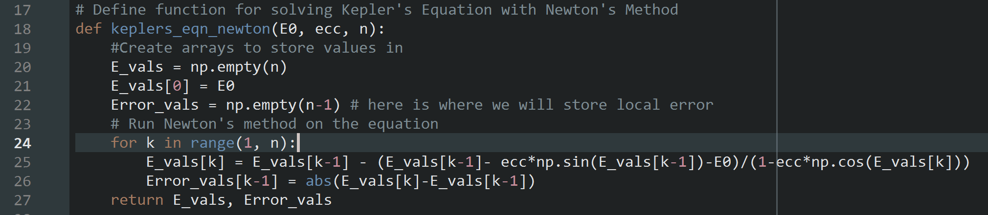
We define a function that takes the previous inputs of _ M, ecc, and n. The function begins by defining two arrays in which we will store our data. The first is where we store our values of $E$ for each iteration and the second is where we store the local error between iterations. This is simply the difference between the iteration we are on and the previous one performed. We let our initial guess for $E$ be $M$. Welch Labs does a good job in his video showing visually how this works better than any other guesses (say, $\frac{M}{2}$ for example). Then, we create a for loop which runs for our specified number of iterations, simply applying the fixed point iteration process and storing each data point in the $E$ values array. We also take the magnitude of the difference between the current iteration and the previous one and store it in our local error array. This can be seen in the code below.

Then, as seen starting at line 30 in the image above, the function is ran and assigned to the variable E_vals which will store both the $E$ values array and error values array. We take the array of our $E$ values and convert them back into degrees as well as round them a bit. We won't need a tremendous amount of precision and this will help keep the displayed data clean. A zero is appended to the front of the local error array too for the sake of displaying the data nicely. This could have just been done within the function by defining the array to be of size n and setting errs[0] = 0. It's all the same at the end of the day since I don't really care about memory allocation or anything like that.

Next, we want to use that pandas library we imported to give us a user-friendly table of data in the console. The two data arrays are combined into one bigger array that can be given to the pandas DataFrame tool. The rows are labeled with an array of two strings "E values" and "Local Error." The columns are numbered $0,1,2,\dots ,n$ to show each iteration. Then, this is all passed into the DataFrame and assinged to a variable. Finally, that just needs to be printed to the console. Now, you may have noticed I also included in the pd.DataFrame options the setting dtype = object. This suppressed the use of scientific notation for the results, since 8.9731e+01 is an ugly way to just say $89.731$.

Great! That is all it takes to solve this problem numerically. If we use the numbers Welch Labs uses in his video, we can take

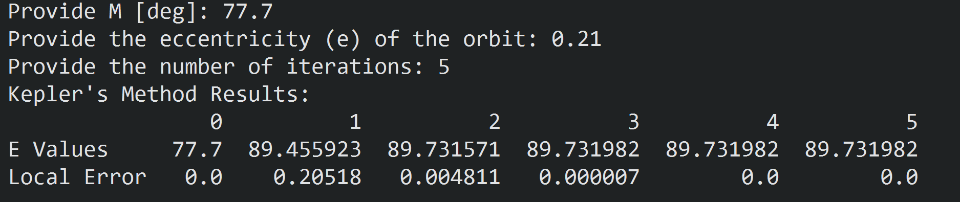
Notice here how the local error here falls off to zero on the last two iterations. Now, of course, there is still error in the small, but with the truncation we performed there is no error in the large! In fact, according to John D. Cook's blog, Kepler only used two iterations and called it good. So this is a highly effective iteration scheme for large objects like planets. I'd also like for you to notice how quickly the error decays away. By the third iteration our error was of order ${10}^{-6}$! We will be comparing this to the Newton-Raphson method.

The Newton-Raphson Method

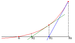
If you've had a course of single variable calculus, you have probably seen the Newton-Raphson method. This is a numerical analysis scheme for finding the roots of an equation iteratively. In this case we would want to find the values of $E$ that get closer and closer to satisfying the equation $M-E+e\sin (E)=0.$ The method can be described by $$x_{n+1}=x_n-\frac{f(x_n)}{f^{\prime }(x_n)}.$$ I think the below image from Wikipedia does a great job of visualizing this method.

We basically code the inputs identical to how we had them before. The function for the iterative method on the other hand is a little different, which you can examine below. Here we set up the iterative fixed point iteration using the Newton-Raphson scheme above (line 25 in the code below). I actually made an error here which gave me poor convergence results. I'll discuss that later as a cautionary tale.

We also use the same DataFrame tool from pandas to display the results. If you want to see the whole code for this one, it is also available at the Github link from the beginning of this entry. Now, I will run 5 iterations with the same mean anomaly and eccentricity values as above. This gives us the result below.

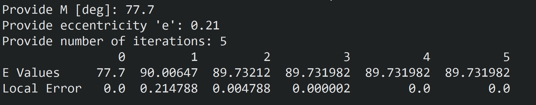
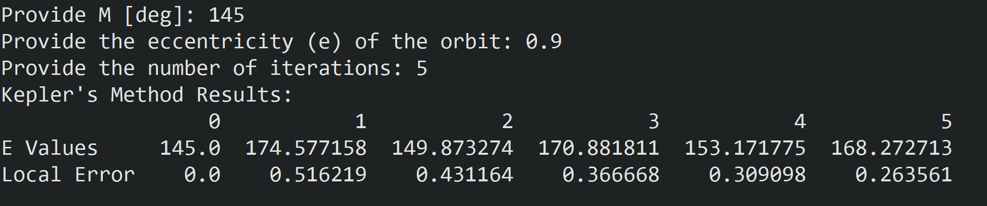
What is different here from Kepler's method? We should immediately be seeing that the local error decays a bit quicker than Kepler's method. At the third iteration the local error is still of order ${10}^{-6}$, but the difference between the two methods is around $5\times {10}^{-6}$. Not a lot, but this is factually a lower local error. These numerical schemes don't always behave the same for different inputs though. Some are more resilient to blowing up (giving results that go to infinity) or taking many more iterations to solve, while others can struggle to converge given certain inputs. For instance, let's use the following inputs

We will still use 5 iterations to make the comparison fair. Below are the results for Kepler's Method:

And here are the results for the Newton-Raphson Method:

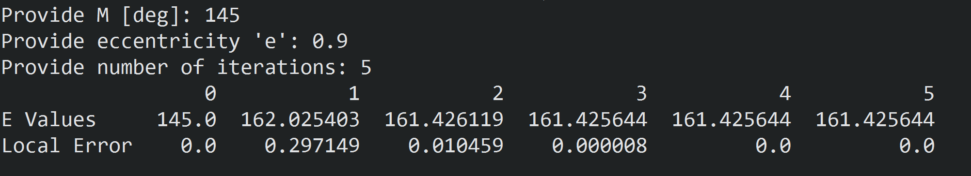
See how Kepler's method bounces around and continues to have local error around the first decimal place? Now look at the results from Newton-Raphson. The method still has local error of order ${10}^{-6}$ on the third iteration! This method is clearly much more stable for various inputs. Welch Labs has a wonderful heat map of error for different values of $M$ and $e$ in his video at 08:41.

Watch Your Indices

Finally, I just wanted to talk about an error I ran into while writing this. I was using the Newton-Raphson Method with the function defined below.

Can you see the problem? The index in the cosine term is $k$ and not $k-1$! This trip up was giving me slower convergence than Kepler's Method. I was looking online for an explanation and couldn't find anything about convergence issues with Newton's method as applied to Kepler's equation. I was writing up a piece about how odd it was and how I couldn't figure out why this equation would behave worse under more sophisticated numerical methods. But, finally I noticed that one little index and as soon as I changed it the method began to converge as Welch Lab's describes in his video. Point being, always read every line of code. No, every character!

--- Self-Teaching Differential Geometry (Journal) ---

08/19/2024

I've recently began trying to learn differential geometry using a couple books and some online notes. I've had the book Differential Geometry in Physics by Gabriel Lugo (can be found here) on my bookshelf for a long time and always thought I'd just use that. I started to take read it and take notes, but quickly ran into some things I disliked. For one, it doesn't have any exercises at the end of the sections/chapters. Also, there are numerous grammatical errors within the first 15 pages and the author makes references to material that has yet to be introduced. I feel that the definitions are not very well motivated and further obfuscated by these remarks regarding more advanced material the reader has yet to see. I haven't totally written the book off, but I opted to study primarily out of another text.

I found a great deal on a hardcover copy (with dust jacket!) of A Course in Differential Geometry and Topology by A. Mishchenko and A. Fomenko from Mir Publishers Moscow. It was a serious treat to be able to get a book from Mir Publishers in hardcover, since so many of these tend to command quite the premium. For anyone interested, many of the titles are available online at the Internet Archive here. The text I am using can be found here. The authors write in a very clear way, using (from what I can tell) mostly standard notation, and they provide many examples. I appreciate the lengths they go to in emphasizing the lessons the reader should draw from the examples. The text also has some exercises, but I have not gotten to the point of attempting any of them. There is a separate problem book to accompany this text as well, but I haven't looked into it. It's also available on the Archive.

I have also been able to find an assortment of online notes to supplement my book, and one set I was able to get printed off, three-hole punched, and put in a binder. To me, a physical copy in my hands will always be superior to a PDF. One thing I have noticed though is I haven't been able to find a lecture series on YouTube that covers diff geo from the perspective of an advanced undergrad/early grad student. I want more than just computational-based differential geometry of curves and surfaces (some discussion of tensor products, manifolds, etc. would be nice), but those topics tend to be found in lectures at the "600 level", i.e., for those a couple years into a Ph.D.

08/26/2024

I've continued to study from the Mir book, but retired Lugo's book. I will need to look through it again, but I am not sure if I even want to keep it. Perhaps it would be best donated to the Richard Sprague Undergrad Lounge at ISU for someone else to find use from it. The first chapter of the Mir book focuses on curvilinear coordinate transformations in Euclidean domains. Typically, the author will use examples from polar, cylindrical, and spherical coordinate transformations. That is, transforming from Cartesian coords. to those systems. The studying was mostly smooth sailing until getting to the construction of the matrix representation of the metric tensor $g_{ab}$ (or in their notation, $g_{mp}$). They began by exploring the arc length of a parameterized curve under coordinate transformation. From this, they rearranged a double sum into a matrix of functions (the inner product of the partials of the coordinate transformation functions). This took me a while to parse. The notation was a bit opaque for me, but after expanding out the terms and seeing how the sums of products of partials rearrange, I was able to understand the formulation. Following this they introduced the Einstein summation notation, but didn't acknowledge it as such. This is a quirk I've found in old Soviet books, where they will omit or rephrase certain known mathematical entities to favor the USSR. For instance, in one of the books I found (I cannot remember which) they refer to the Euler-Lagrange equation as the Ostrogradsky Equation (the context was not related to Gauss's Theorem, which is alternatively known as Ostrogradsky's Theorem. Wikipedia).

In order to supplement the Mir text, I also got a copy of Erwin Kreyszig's Differential Geometry. This one is focused on curves and surfaces in 3-D, and perhaps has a less theoretical approach, but I thought this would be a good way to ground the content I was reading in the other one. A major plus with the Kreyszig book is that he has solutions for, I believe, all of the problems in the book! That is a huge help when self-studying. I have yet to do the problems from Chapter 1 of the Mishchenko and Fomenko book, but they don't look too crazy.

10/08/2024

I've placed my differential geometry studies on hold in favor of something a bit more palatable. I think the text I was using started off with complete generality, which made it harder to follow and lead me to get bored with it. Also, as I've been getting off escitalopram the withdrawal symptoms have made it much harder to focus and tackle challenging material. Instead, I've opted to study John R. Taylor's Classical Mechanics, which is much more reader friendly and the content is familiar enough to me so that I stick with it. Eventually I will come back to differential geometry, but for now it is on an indefinite pause.

--- Venn Diagram of Mathematical Spaces ---

Originally posted by the mathematician Anthony Bonato on Twitter, I thought this image was particularly illustrative of the relationship between topological spaces, metric spaces, and vector spaces. I particularly enjoy studying the properties of the $L^2$ space.

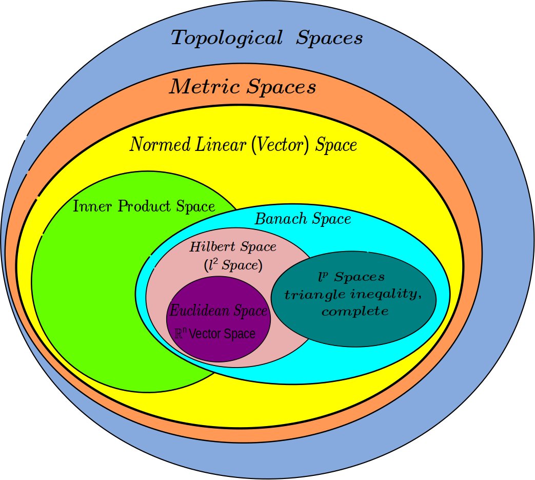
I was able to find this post as a source for the image.

--- Calculus of Variations Seminar Presentation ---

Below are slides for a presentation I prepared for the Junior Analysis Seminar at Iowa State University. Here is the presentation itself (redirects to YouTube).

--- Calculus of Variations Project ---

*** UNDER CONSTRUCTION ***

As part of the Iowa State Mathematical Research Teams (ISMaRT), I worked on an undergraduate research project intended to give undergrads a look at what the mathematical research process was like. I worked with two other math students (who I knew from the ISU Math Club) on generalized versions of the brachistochrone problem. The research itself wasn't anything novel, but surprisingly enough I did find myself running into dead ends where there was either scant resources or, in an exciting way, no resources at all. The literature on the brachistochrone problem itself is plentiful, but various twists on the idea can quickly place someone in much less charted waters. I think this showed me firsthand what it means to be creative in the research process. Some of the versions I found were quite unique. For instance, I was reading a paper from a US Naval Academy physics researcher on what he dubbed the "electrobrachistochrone," where a charged particle moves on a frictionless track under some electrostatic force (as opposed to the usual mass influenced by gravity along a frictionless path).

The project involved several presentations to the two post-docs supervising us on our progress/hurdles we encountered. They were both very keen on providing a more in-depth understanding of the "why" of variational problems, which I appreciated. One of the problems they posed to us was how the brachistochrone will behave compared to a linear or parabolic trajectory. Also, the two coordinators of the project (with whom the post-docs collaborated with on research) asked about the behavior of the brachistochrone as the endpoint tended to infinity. How would the time vary? How would arc length vary? These sort of questions. Some other problems were posed, which I can delve into further at a later time. When it came to deliverables, I took on the role as the numerical analyst for the project. I used MATLAB to simulate the behavior of these different curves and to try and gain some insight into how they behave (which could inform any analytical problem solving attempts). The post-docs said there was a way of dealing with the problems analytically, but I wasn't able to find a good avenue to pursue with that.

*** UNDER CONSTRUCTION ***

Contact Me | OpenPGP Key